Computing Quadratic Integer Relations

Newcastle, NSW, December 7–10th 2021
For convenience, we will usually think of \( x \in \) \( \RR^n \) and \( a \in \) \( \ZZ^n \) and say that \( a \) is an integer realtion of \( x \).
For convenience, we will usually think of \( x \in \) \( \CC^n \) and \( a \in \) \( \ZZ[i]^n \) and say that \( a \) is an integer realtion of \( x \).
When talking about integer relations in general, we use the following notation so as to encapsulate all cases.
We will use \( \FF \) to denote the field of numbers which we are relating and we will use \( \mathcal{O} \) to denote the ring of integers from which the relation elements are from.
The previous definitions we call the classical cases. That is, when \( \mathcal{O} = \ZZ \), \( \FF = \RR\), and when \( \mathcal{O} = \ZZ[i] \), \( \FF = \CC \).
An information theoretic argument shows that in order to numerically compute an integer relation on \( n \) numbers, where the relation consists of integers with no more than \( d \) digits, then at least \( nd \) decimal digits of precision need to be used.
In the case of complex numbers and Gaussian integers, the number of digits is the number of digits in the real part, or the imaginary part, whichever is larger.
- LLL (indirectly)
- PSLQ (directly)
LLL
The LLL algorithm was introduced by Lenstra, Lenstra Jr, and Lovasz in 1982.
It is not an algorithm for computing integer relations directly. Instead it finds short lattice vectors
It can, however, be used to compute integer relations
LLL
Let \( B = \left\{ b_1, \dotsc, b_n\right\} \subset \FF^n \) be a linearly independent set of vectors. The set \[ L = \left\{ \lambda_1 b_1, \dotsc, \lambda_n b_n : \lambda_1 \in \mathcal{O} \right\} \] is the lattice spanned by \(B\). We call \( B \) the basis of the lattice \( L \)
We will sometimes refer to an \( \mathcal{O} \)-lattice if we need to specify the integer ring explicitly.
LLL
Given a basis \( B \) for a lattice \( L \), the LLL algorithm computes a basis \( B^\prime = (b^\prime_1,\dotsc,b^\prime_n) \) such that \[ \begin{gather} \lvert \mu_{i,j} \rvert \le \frac{1}{2} \text{ for } 1 \le j < i \le n \\ \lvert\lvert b^*_i + \mu_{i,j} b^*_{i-1} \rvert\rvert^2 \ge \frac{3}{4} \lvert\lvert b^*_{i-1} \rvert\rvert^2 \text{ for } 1 < i \le n \\ \end{gather} \] where \( b^*_i = b^\prime_i - \sum_{j=1}^{i-1}\mu_{i,j}b^*_j \text{ and } \mu_{i,j} = \frac{ b^\prime_i \cdot b^*_j}{\lvert\lvert b^*_j \rvert\rvert^2} \)
LLL
To find an integer relation on \( x = (x_1, \dotsc, x_n) \in \RR^n \) we can use LLL on the lattice \[ L := \begin{bmatrix} 1 & 0 & 0 & \dotsm & 0 & Nx_1 \\ 0 & 1 & 0 & \dotsm & 0 & Nx_2 \\ \vdots & \vdots & \ddots & \dotsm & \vdots & \vdots \\ 0 & 0 & 0 & \dotsm & 1 & Nx_n \end{bmatrix}\] for some \( N \in \RR \).
Think of this as the augmented matrix \( \left[ I_n\, Nx \right] \).
LLL
Elements of the lattice look like \[ \left(\lambda_1, \dotsc, \lambda_n, N(\lambda_1x_1 + \dotsm + \lambda_nx_n) \right) \] So if the \( \lambda_i \) are an integer relation for \( x \) then the last term will be 0.
We can prove that if \( N \) is large enough, then the first element of the reduced lattice must contain the integer relation.
LLL
For the complex case where n \( z = (z_1, \dotsc, z_n) \in \CC^n \) we still use the augmented lattice \( L := \left[ I_n \, Nz \right] \) like we did for the real case.
However we then construct a 2nd augmented lattice \[ \begin{bmatrix} \Re{L} & \Im{L} \\ -\Im{L} & \Re{L}\end{bmatrix} \] and use LLL on that lattice.
As with the real case, so long as \( N \) is large enough then the procedure must find an integer relation.
LLL
In all cases, we don't know how large to make \( N \) before we start. So we must use trial and error.
We have found, experimentally, that with numeric (floating point) calculations it is possible for \( N \) to be too large, even though the theory requires \( N \) to be “sufficiently large”.
PSLQ
The PSLQ algorithm was introduced by Ferguson & Bailey in 1988. It was later analysed by Ferguson, Bailey, and Arno in 1999
It can handle both the real and complex cases directly.
We will not discuss the details of the algorithm itself. However we will establish some facts.
PSLQ
Observe that in both the real and complex cases \( \mathcal{O} \) forms a lattice, and that \( \mathcal{O} \subset \FF \).
Let \( x \in \FF \). An integer \( a \in \mathcal{O} \) is a nearest integer if \( \lvert x-a \rvert \) is maximal. A function \( \lceil \cdot \rfloor : \FF \to \mathcal{O} \) is a nearest integer functino if it maps each \( x \in \FF \) to one of its nearest integers.
We denote by \( \lceil \cdot \rfloor_{\mathcal{O}} \) if we need to be specific.
PSLQ
There are parameters: \( \gamma, \rho \), and \( \tau \) that must satisfy \[ \begin{gather} \frac{1}{\rho} \ge \lvert x - \lceil x \rfloor \rvert \text{ for all } x \in \FF \\ 1 < \tau \le \rho \\ \frac{1}{\tau^2} = \frac{1}{\gamma^2} + \frac{1}{\rho^2} \end{gather} \]
\( \rho \) is bounded by the integer lattice; choose to minimise \(1/\rho\).
\( \gamma \) is minimised when \( \tau = 1 \); choose any larger value.
\( \tau \) is fixed by the choice of \( \gamma \) and the value of \( \rho \).
PSLQ
Each iteration of the PSLQ algorithm finds an increased lower bound on the norm of any integer relation on the input.
The algorithm can terminate when that bound exceeds some threshold.
If the algorithm finds a relation, \( a \) then \( \lvert\lvert a \rvert\rvert \le \gamma^{n-2}M \) where \( M \) is the norm of the smallest possible relation.
PSLQ
In Principle:
- We give PSLQ:
- The numbers we wish to find a relation for.
- An upper bound, \( b \), for the Euclidean norm of the relation we wish to find.
- PSLQ gives either:
- A relation, \( a \) where \( \norm{a} \le b \) and \( \norm{a} \le \gamma^{n-2}M \).
- A declaration that no such relation exists.
In Practice:
Due to floating point arithmetic and speed optimisations.
- We give PSLQ:
- The numbers we wish to find a relation for
- PSLQ gives:
- A relation accurate to the calculation precision with no bound guarantee.
Comparing LLL and PSLQ
- PSLQ is designed specifically for integer relation compuation
- In experimental testing:
- PSLQ required lower precision than LLL (for the same relation).
- PSLQ took less time than LLL (for the same relation).
Algebraic Number Theory
Let \( \FF \) be a field. If \( \FF \) is a subfield of some other field \( \KK \) (i.e., \( \FF \subseteq \KK \) then we call \( \KK \) a field extension (or, equivalently an extension field) of \( \FF \).
We denote this by \( \KK:\FF \) when we need to be explicit about the base field and the extension.
Note that the literature often uses the notation \( \KK/\FF \) instead.
Algebraic Number Theory
Let \( \FF \) be a field, and consider an extension field \( \KK:\FF \). An element \( k \in \KK \) is said to be algebraic over \( \FF \) if it satisfies \[ f_nk^n + \dotsm + f_1 k + f_0 = 0 \] for some \( n \in \NN \) and \( f_i \in \FF \). Note that \( f_n \ne 0 \).
For example \( \sqrt{2} \) satisfies \( k^2 - 2 = 0 \) and so is algebraic over the rationals.
Algebraic Number Theory
Let \( D \) be an integral domain and consider an extension field \( \KK:\FF \) such that \( D \subseteq \KK \). An element \( k \in \KK \) is said to be integeral over \( \FF \) if it satisfies a monic polynomial \[ k^n + d_{n-1}k^{n-1} + \dotsm + d_1 k + d_0 = 0 \] for some \( n \in \NN \) and \( d_i \in D \)
An integral domain is a commutative ring with multiplicative identity and no non-zero elements \( d_1, d_2 \) with the property that \( d_1d_2 = 0 \).
Algebraic Number Theory
Let \( z \in \CC \).
We denote by \( \QQ(z) \) the smallest subfield of \( \CC \) that contains both \( \QQ \) and \( z \).
We denote by \( \ZZ[z] \) the smallest subring of \( \CC \) that contains both \( \ZZ \) and \( z \).
Note that the ring \( \ZZ \) is often called the “rational integers” to avoid ambiguity.
Algebraic Number Theory
We are primarily interested in extension fields of \( \QQ \).
A number \( z \in \CC \) is an algebraic number (or simply algebraic) if it is algebraic over \( \QQ \).
A number \( z \in \CC \) is an algebraic integer if it is integral over \( \ZZ \).
The ring of all algebraic integers is denoted by \( \mathcal{A} \).
An algebraic extension is real if \( \KK \subseteq \RR \) and complex otherwise.
Algebraic Number Theory
We are primarily interested in extension fields of \( \QQ \).
An extension field \( \KK:\QQ \) is an algebraic extension field (or simply an algebraic extension if every \( k \in \KK \) is an algebraic number.
Its ring of integers of \( \KK \), denoted \( \mathcal{O}_{\KK} \), is \( \KK \cap \mathcal{A} \). We call such rings algebraic integers
Quadratic Fields
We will restrict our attention to quadratic extension fields. These are fields of the form: \[ \QQ( \sqrt{D} ) = \left\{ q_1 + q_2 \sqrt{D} : q_i \in \QQ \right\} \] wher \( D \in \ZZ \) is square free.
Elements of these fields satisfy quadratic (or lower degree) polynomials with rational coefficients.
Quadratic Fields
The algebraic integers of a quadratic field (which we call quadratic integers) are of the form \[ \mathcal{O}_{\QQ(\sqrt{D})} = \ZZ[\omega] = \left\{ m_1 + m_2 \omega : m_i \in \mathbb{Z} \right\} \] where \[ \omega = \begin{cases} \sqrt{D} & \text{ if } D \equiv 2,3 \;(\operatorname{mod} 4) \\ \frac{1+\sqrt{D}}{2} & \text{ if } D \equiv 1 \;(\operatorname{mod} 4) \end{cases} \]
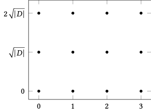
\( D \equiv 2,3 \;(\operatorname{mod} 4) \)
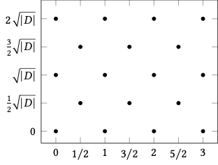
\( D \equiv 1 \;(\operatorname{mod} 4) \)
Quadratic Fields
Finally we mention a special class of quadratic fields.
Relations With Algebraic Integers
Recall the definiton of an integer relation:
Relations With Algebraic Integers
For relations of algebraic integers we specify an intermediate extension field.
Let \( \FF \in \{ \RR, \CC \} \) and let \( \KK \) be an algebraic extension field. Let \( \mathcal{O} = \mathcal{O_{\KK}} \).
Let \( x_1, \dotsc, x_n \in \FF \). Integers, \( a_1, \dotsc, a_n \in \mathcal{O} \) are an algebraic integer relation (or a \( \KK \)-integer relation) of the original numbers \( x_i \) if \[ a_1x_1 + \dotsm + a_nx_n = 0 \]
Reduction to Classical Cases
Observe that for an quadratic integer relation: \[ \begin{align*} & \left(m_{1,1} + m_{1,2} \omega\right)\,x_1 + \dotsm + \left(m_{n,1} + m_{n,2}\omega\right)\,x_n \\ =& \left(m_{1,1}x_1 + \dotsm + m_{n,1}x_n \right) + \left(m_{1,2}\, \omega x_1 + \dotsm m_{n,2}\,\omega x_n\right) \end{align*} \]
This suggests a way to reduce a quadratic integer relation to a classical one.
Reduction to Classical Cases
Given \( (x_1, \dotsc, x_n) \in \FF^n \) we construct \( (x_1, \dotsc, x_n, x_1\omega, \dotsc, x_n\omega) \in \FF^{2n} \) and search for a classical integer relation on that.
We recover the integer relation by taking \( a_k + a_{n+k}\omega \) for \( 1 \le k \le n \).
This works well for real quadratic fields (i.e., when \( D > 1 \)). It works less well for complex quadratic fields.
Reduction to Classical Cases
In the complex case, the integers are of the form \( a_k = m_{k,1} + m_{k,2} i \). So when we attempt to recover the relation we get \[ \left(m_{k,1} + m_{k,2} i\right) + \left(m_{k+n,1} + m_{k+n,2} i \right)\omega \] after expansion and some simplification we get \[ \alpha_1 + \beta_2 i \sqrt{\lvert D \rvert} + \alpha_2 i - \beta_2 \sqrt{\lvert D \rvert} \text{ for } \alpha_1, \beta_1 \in \ZZ \] which is not an algebraic integer in \( \QQ(\sqrt{D}) \) if \( \alpha_2 \ne 0 \) or \( \beta_2 \ne 0 \).
Reduction to Classical Cases
Much of the time the reduction technique works fine, and gives good answers even in the complex cases.
When it does not work, we try two techniques to nonetheless extract a relation.
Reduction to Classical Cases
Decomposition method
We observe that \[ \alpha_1 + \beta_2 i \sqrt{\lvert D \rvert} + \alpha_2 i - \beta_2 \sqrt{\lvert D \rvert}\] can be written as \[ \left( \alpha_1 + \beta_2 i\sqrt{\lvert D \rvert} \right) + i \left( \alpha_2 + \beta_2 i\sqrt{\lvert D \rvert} \right) \] and we have two possible algebraic integers embedded. We try extracting only these.
Reduction to Classical Cases
Conjugate Method
Given \[ \alpha_1 + \beta_2 i \sqrt{\lvert D \rvert} + \alpha_2 i - \beta_2 \sqrt{\lvert D \rvert} \] a conjugate is \[ \alpha_1 - \beta_2 i \sqrt{\lvert D \rvert} - \alpha_2 i - \beta_2 \sqrt{\lvert D \rvert} \]
Multiplying the number by its conjugate gives an element of \( \mathcal{O}_{\QQ(\sqrt{D})} \). We multiply all elements of the relation by the conjugate of only one of the elements.
Reduction to Classical Cases
Both the methods for correcting the complex case work well in practice.
We do not have proofs that they will always be correct. It is nonetheless easy to just try them, and check the extracted relation.
Using LLL
To compute an algebraic integer n \( z = (z_1, \dotsc, z_n) \in \FF^n \) we still use the augmented lattice \( L := \left[ I_n \, Nz \right] \) like we did for the real case.
However we then construct a 2nd augmented lattice. \[ \begin{bmatrix} \Re{L} & \Im{L} \\ \mathfrak{W_1}{L} & \mathfrak{W_2}{L}\end{bmatrix} \] and use LLL on that lattice.
Using LLL
However we then construct a 2nd augmented lattice. \[ \begin{bmatrix} \Re{L} & \Im{L} \\ \mathfrak{W_1}{L} & \mathfrak{W_2}{L}\end{bmatrix} \] and use LLL on that lattice.
\[ \mathfrak{W_1}{x_k} = \begin{cases} -\sqrt{\lvert D \rvert} \Im{x_k} & \text{ if } \text{ if } D \equiv 2,3 \;(\operatorname{mod} 4) \\ \left(\Re{x_k} - \sqrt{\lvert D \rvert}\Im{x_k} \right)/2 & \text{ if } D \equiv 1 \;(\operatorname{mod} 4) \end{cases} \] \[ \mathfrak{W_2}{x_k} = \begin{cases} \sqrt{\lvert D \rvert} \Re{x_k} & \text{ if } \text{ if } D \equiv 2,3 \;(\operatorname{mod} 4) \\ \left(\Im{x_k} + \sqrt{\lvert D \rvert}\Re{x_k} \right)/2 & \text{ if } D \equiv 1 \;(\operatorname{mod} 4) \end{cases} \]
Using LLL
As with the other cases, so long as \( N \) is large enough then the procedure must find an algebraic integer relation.
Modifying PSLQ
We attempt to modify PSLQ while keeping the existing theory.
We simply use a quadratic integer nearest integer function, and modify the algorithm to allow us to specify the quadratic extension field we wish to use.
Modifying PSLQ
We simply use a quadratic integer nearest integer function, and modify the algorithm to allow us to specify the quadratic extension field we wish to use.
This introduces a problem: for real quadratic extension fields, the integers do not form a lattice (there is no unique nearest integer to a field element), so we cannot use the existing theory.
We restrict our attention to the complex cases, then.
Modifying PSLQ
We restrict our attention to the complex cases, then.
In these cases we have a more subtle problem.
As \( D \) increases, the parameter \( \rho \) decreases, until eventually \( \rho < 1 \) making it impossible to satisfy the \( 1 < \tau \le \rho \) condition.
Modifying PSLQ
In these cases we have a more subtle problem.
As \( D \) increases, the parameter \( \rho \) decreases, until eventually \( \rho < 1 \) making it impossible to satisfy the \( 1 < \tau \le \rho \) condition.
The complex quadratic fields that do not exhibit these problems are exactly: \[ \QQ(\sqrt{-2}), \QQ(\sqrt{-3}), \QQ(\sqrt{-7}), \QQ(\sqrt{-11})\]
Modifying PSLQ
As \( D \) increases, the parameter \( \rho \) decreases, until eventually \( \rho < 1 \) making it impossible to satisfy the \( 1 < \tau \le \rho \) condition.
The complex quadratic fields that do not exhibit these problems are exactly: \[ \QQ(\sqrt{-2}), \QQ(\sqrt{-3}), \QQ(\sqrt{-7}), \QQ(\sqrt{-11})\]
These are precisely the complex quadratic norm Euclidean fields.
Modifying PSLQ
The complex quadratic fields that do not exhibit these problems are exactly: \[ \QQ(\sqrt{-2}), \QQ(\sqrt{-3}), \QQ(\sqrt{-7}), \QQ(\sqrt{-11}) \]
We note that we've had surprising success with the modified PSLQ on \[ \QQ(\sqrt{-5}), \QQ(\sqrt{-6}), \QQ(\sqrt{-10}) \] even though they do not fit the existing theory.